Unknown macro: {float}
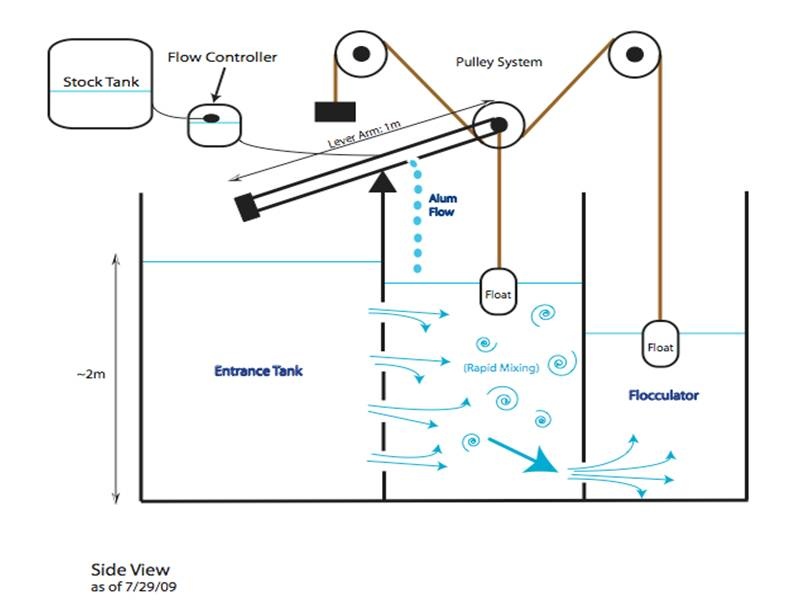
Illustration of non-linear chemical doser
Introduction
The non-linear dose controller was redesigned in order to reduce the amount of aeration caused as water traveled through the plant. For more information about the theory of the non-linear dose controller see the page for the original non-linear CDC design.
Methods
Sizing the Orifice
The orifice between the rapid mix and flocculation tanks is designed to produce a difference in water level high that can then be sensed by a float which would then change the flow rate of aluminum sulfate:
No Latex value
No preview is available, please have your Latex markup text selected when inserting the Latex macro or click edit on an existing Latex macro when text is present to preview the rendered result.
Example Markup
\begin{eqnarray}
    y&=&ax^{2}+bx+c \nonumber\\
    E&=&mc^2 \nonumber\\
    {\delta y \over \delta x}
        &=& {{a\over b}\over c}
\end{eqnarray}
Example Render

For more information about Latex, you can find in the following documentation LaTeX Plugin
where
No Latex value
No preview is available, please have your Latex markup text selected when inserting the Latex macro or click edit on an existing Latex macro when text is present to preview the rendered result.
Example Markup
\begin{eqnarray}
    y&=&ax^{2}+bx+c \nonumber\\
    E&=&mc^2 \nonumber\\
    {\delta y \over \delta x}
        &=& {{a\over b}\over c}
\end{eqnarray}
Example Render
For more information about Latex, you can find in the following documentation LaTeX Plugin
is the difference in head loss between the rapid mix and flocculation tank- K orifice is the required minor loss coefficient through the orifice
- V jet is the velocity in the dosing tube
This head loss was then used to determine the velocity of the water through the orifice and the residence time. Using the following equations:
Velocity of Jets:
No Latex value
No preview is available, please have your Latex markup text selected when inserting the Latex macro or click edit on an existing Latex macro when text is present to preview the rendered result.
Example Markup
\begin{eqnarray}
    y&=&ax^{2}+bx+c \nonumber\\
    E&=&mc^2 \nonumber\\
    {\delta y \over \delta x}
        &=& {{a\over b}\over c}
\end{eqnarray}
Example Render
For more information about Latex, you can find in the following documentation LaTeX Plugin
where
- V jet is the velocity of the jet
- Q is the flow rate through the system
- C d is the vena contracta coefficient for exit condition in orifice
- A orifice is the area of the orifice
Residence time :
No Latex value
No preview is available, please have your Latex markup text selected when inserting the Latex macro or click edit on an existing Latex macro when text is present to preview the rendered result.
Example Markup
\begin{eqnarray}
    y&=&ax^{2}+bx+c \nonumber\\
    E&=&mc^2 \nonumber\\
    {\delta y \over \delta x}
        &=& {{a\over b}\over c}
\end{eqnarray}
Example Render
For more information about Latex, you can find in the following documentation LaTeX Plugin
where
No Latex value
No preview is available, please have your Latex markup text selected when inserting the Latex macro or click edit on an existing Latex macro when text is present to preview the rendered result.
Example Markup
\begin{eqnarray}
    y&=&ax^{2}+bx+c \nonumber\\
    E&=&mc^2 \nonumber\\
    {\delta y \over \delta x}
        &=& {{a\over b}\over c}
\end{eqnarray}
Example Render
For more information about Latex, you can find in the following documentation LaTeX Plugin
is the residence time
- d orifice is the diameter of the orifice
- V jet is the velocity of the jet
Once these values were determined, we were able to calculate the energy dissipation rate using the following equation:
No Latex value
No preview is available, please have your Latex markup text selected when inserting the Latex macro or click edit on an existing Latex macro when text is present to preview the rendered result.
Example Markup
\begin{eqnarray}
    y&=&ax^{2}+bx+c \nonumber\\
    E&=&mc^2 \nonumber\\
    {\delta y \over \delta x}
        &=& {{a\over b}\over c}
\end{eqnarray}
Example Render
For more information about Latex, you can find in the following documentation LaTeX Plugin
where
No Latex value
No preview is available, please have your Latex markup text selected when inserting the Latex macro or click edit on an existing Latex macro when text is present to preview the rendered result.
Example Markup
\begin{eqnarray}
    y&=&ax^{2}+bx+c \nonumber\\
    E&=&mc^2 \nonumber\\
    {\delta y \over \delta x}
        &=& {{a\over b}\over c}
\end{eqnarray}
Example Render
For more information about Latex, you can find in the following documentation LaTeX Plugin
is the energy dissipation rate- g is gravity
No Latex value
No preview is available, please have your Latex markup text selected when inserting the Latex macro or click edit on an existing Latex macro when text is present to preview the rendered result.
Example Markup
\begin{eqnarray}
    y&=&ax^{2}+bx+c \nonumber\\
    E&=&mc^2 \nonumber\\
    {\delta y \over \delta x}
        &=& {{a\over b}\over c}
\end{eqnarray}
Example Render
For more information about Latex, you can find in the following documentation LaTeX Plugin
is the head loss
No Latex value
No preview is available, please have your Latex markup text selected when inserting the Latex macro or click edit on an existing Latex macro when text is present to preview the rendered result.
Example Markup
\begin{eqnarray}
    y&=&ax^{2}+bx+c \nonumber\\
    E&=&mc^2 \nonumber\\
    {\delta y \over \delta x}
        &=& {{a\over b}\over c}
\end{eqnarray}
Example Render
For more information about Latex, you can find in the following documentation LaTeX Plugin
is the residence time
We sought to keep the energy dissipation rate between .5 and 1 W/kg so that molecular scale diffusion works and in order for small scale turbulent mixing to be effective.
Lever Arm and Float
We first must determine the size of the counterweight on the doser arm in order to ensure that the dosage will only be a function of the difference in water height in the flocculation and rapid mix tanks. The mass of the weight is calculated by determining the mass of the doser when full.
No Latex value
No preview is available, please have your Latex markup text selected when inserting the Latex macro or click edit on an existing Latex macro when text is present to preview the rendered result.
Example Markup
\begin{eqnarray}
    y&=&ax^{2}+bx+c \nonumber\\
    E&=&mc^2 \nonumber\\
    {\delta y \over \delta x}
        &=& {{a\over b}\over c}
\end{eqnarray}
Example Render
For more information about Latex, you can find in the following documentation LaTeX Plugin
where
- D actual is the difference between the given diameter of the dosing tube and the measured diameter of the dosing tube
No Latex value
No preview is available, please have your Latex markup text selected when inserting the Latex macro or click edit on an existing Latex macro when text is present to preview the rendered result.
Example Markup
\begin{eqnarray}
    y&=&ax^{2}+bx+c \nonumber\\
    E&=&mc^2 \nonumber\\
    {\delta y \over \delta x}
        &=& {{a\over b}\over c}
\end{eqnarray}
Example Render
For more information about Latex, you can find in the following documentation LaTeX Plugin
is the density of water
No Latex value
No preview is available, please have your Latex markup text selected when inserting the Latex macro or click edit on an existing Latex macro when text is present to preview the rendered result.
Example Markup
\begin{eqnarray}
    y&=&ax^{2}+bx+c \nonumber\\
    E&=&mc^2 \nonumber\\
    {\delta y \over \delta x}
        &=& {{a\over b}\over c}
\end{eqnarray}
Example Render
For more information about Latex, you can find in the following documentation LaTeX Plugin
is the mass of the doser empty
The size of the float can be determined using a moment balance around the pivot of the lever arm. This is to ensure that a change in head in the entrance tank will cause a similar change in the relative height of the float. The float was sized using the same float sizing algorithm used by the linear CDC. Based on this we found that a float of 13.3 inches would theoretically be able to measure a .25cm height difference.
Conclusion
Based on our calculations, we found that an orifice of 8cm would give us an acceptable energy dissipation rate of .927 W/kg and would require a 13.3in float. This float would have a .25cm sensitivity over a 15.2cm height difference.
Unknown macro: {float}
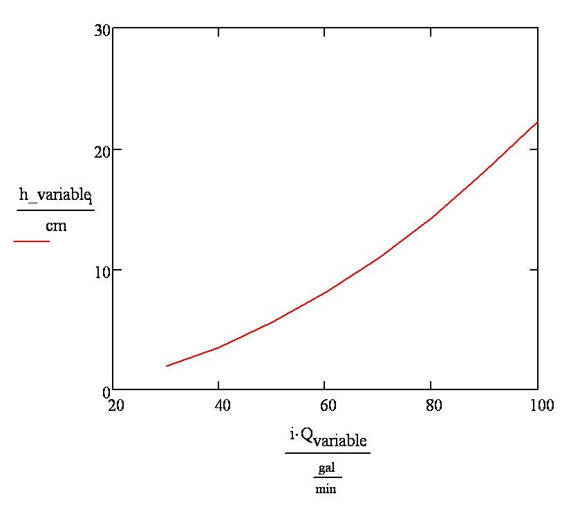
Graph showing the non-linear relationship between the head loss vs. the flow rate through a 8cm diameter orifice
Additionally we found 2 solutions with multiple orifices. We did this because more orifices at a smaller diameter will keep energy dissepation constant while increasing overall headloss across the system. The first solution gave us 8 orifices with a 4.5cm diameter and a minimum energy dissipation rate of .831.
Unknown macro: {float}
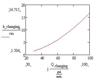
Graph showing the non-linear relationship between the head loss vs. the flow rate through eight 4.5cm diameter orifices
The second solution gave us 175 orifices with a 2 cm diameter and a minimum energy dissipation rate of .496.
Unknown macro: {float}
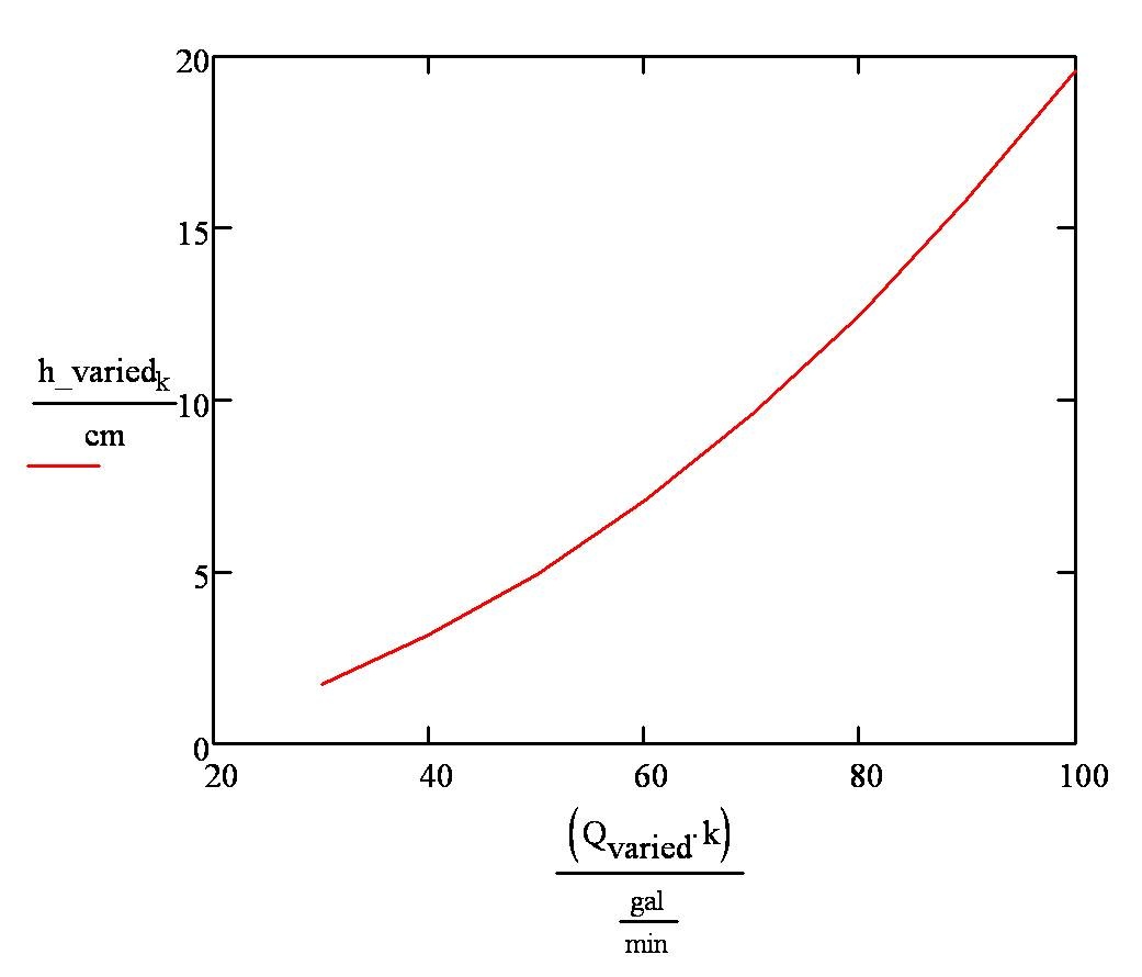
Graph showing the non-linear relationship between the head loss vs. the flow rate through 175 2cm diameter orifices

 user-5ca95, last updated by Anonymous on Sep 08, 2025
3 minute read
user-5ca95, last updated by Anonymous on Sep 08, 2025
3 minute read