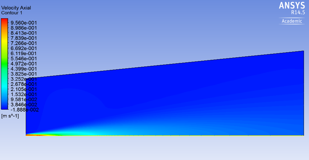
With CFD Post open, go to File-Load Results and select the file that you created on exporting (this is only if you did not already have it open from the previous step). Creating a contour plot of the axial velocity will give you this; you can see that the axial velocity spreads in the X direction.
Plot the axial velocity and turbulent kinetic energy k along the centerline. To do this, go to Insert-Location-Line. Specify the line with two points, one at (0,0,0) and the other at (1,0,0) corresponding to endpoints on the centerline. Create a graph of the axial velocity: select the Chart icon, give the chart a title and press "OK". In the Data Series tab for the chart, select the name of the line that you just created on the centerline in the Location drop down list. Select X as the variable on the X-axis, and Axial Velocity/Turbulent Kinetic energy for the Y variable. Your graphs should look approximately like this:
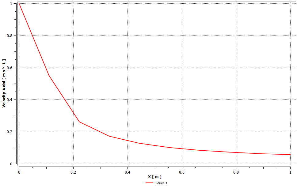
It is clear that the axial velocity decreases with increasing distance from the jet.
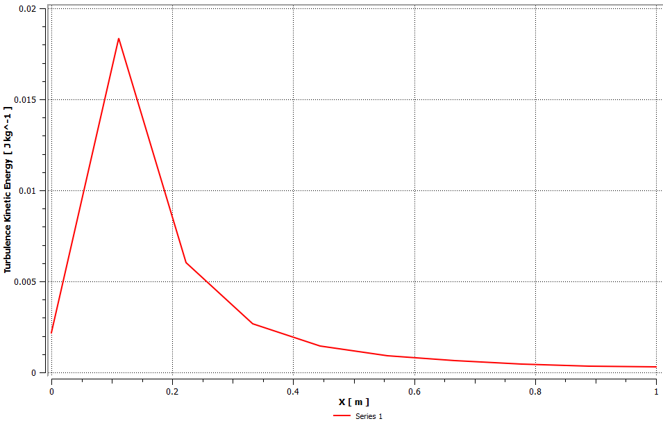
The turbulent kinetic energy is the mean kinetic energy per unit mass in the fluctuating velocity field. It is governed by a production term P, a dissipation term -ε, mean flow convection -Dk/Dt, and turbulent transport -grad(T). The peak in turbulent kinetic energy just after the inlet is due to the production term (affected by fluid shear or friction) dominating; the turbulent kinetic energy again approaches zero as the distance from the inlet increases as the fluid is convected and dissipated away from the centerline into the surroundings.
Go to Step 6. Verification & Validation
Go to all FLUENT Learning Modules