*** This version of Confluence is for testing only and contains a copy of content from June 29th 2026. No changes will be preserved. ***

PDF version of our MATHCAD File.
...
...
Target Input:
This is where the user inputs:
* The plant flow rate (Q)
* Number of granular Filters (N)
* Backwash Time between 5-10 min (Tbw)
* Percent the Sand Bed expands (Texpansion)
Condition Input:
This is where the parameters of the construction materials are entered:
* Diameter of particles, depth of bed, porosity, specific gravity, and d60 of sand and gravel.
* Water Treatment Filtration Rate
* Diameter of backwash orifice, clear well, and piping (which should be moved to fluid functions)
* Roughness and length of piping
* Density, and dynamic and kinematic viscosity of water
Calculations:
First we determine the size of the filter and head loss in normal filtration through the sand and gravel bed.
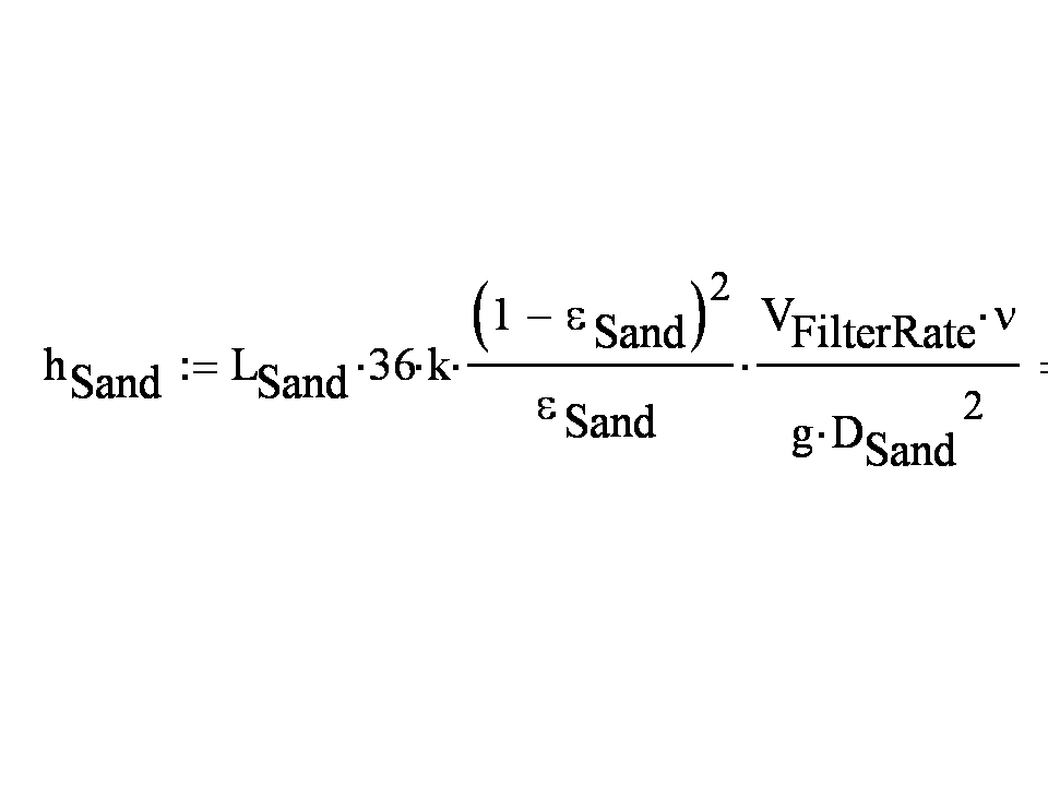
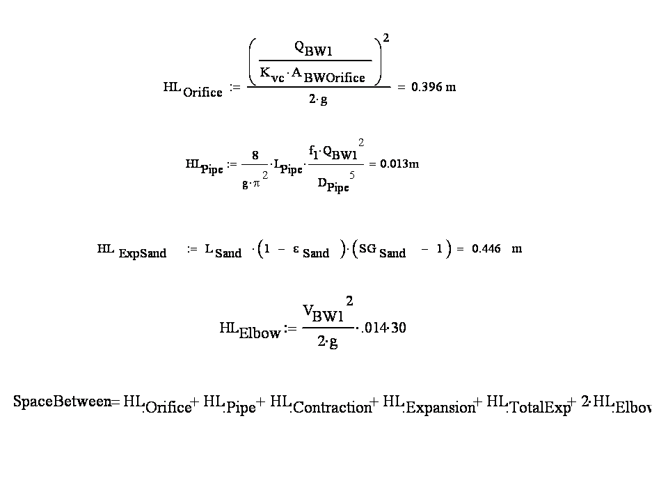
Then we use two approaches to find the area of the clear well . The first is based upon conventional knowledge that the back wash velocity needs to be 10 times the filter velocity. From there we know that the space between the top of the filter bed and the bottom of the clear well is linked directly to the amount of head loss between those two points (head loss from the pipe, elbows, expansion and contraction, expansion of the bed). To do this, we used information from Schulz and Okun (1992).
The second approach is to use the empirical formula, called the Weber Equation. The velocity for filtration is based on the sand's d60 (this equation is meant only for sand) and the specific weight of both water and sand.
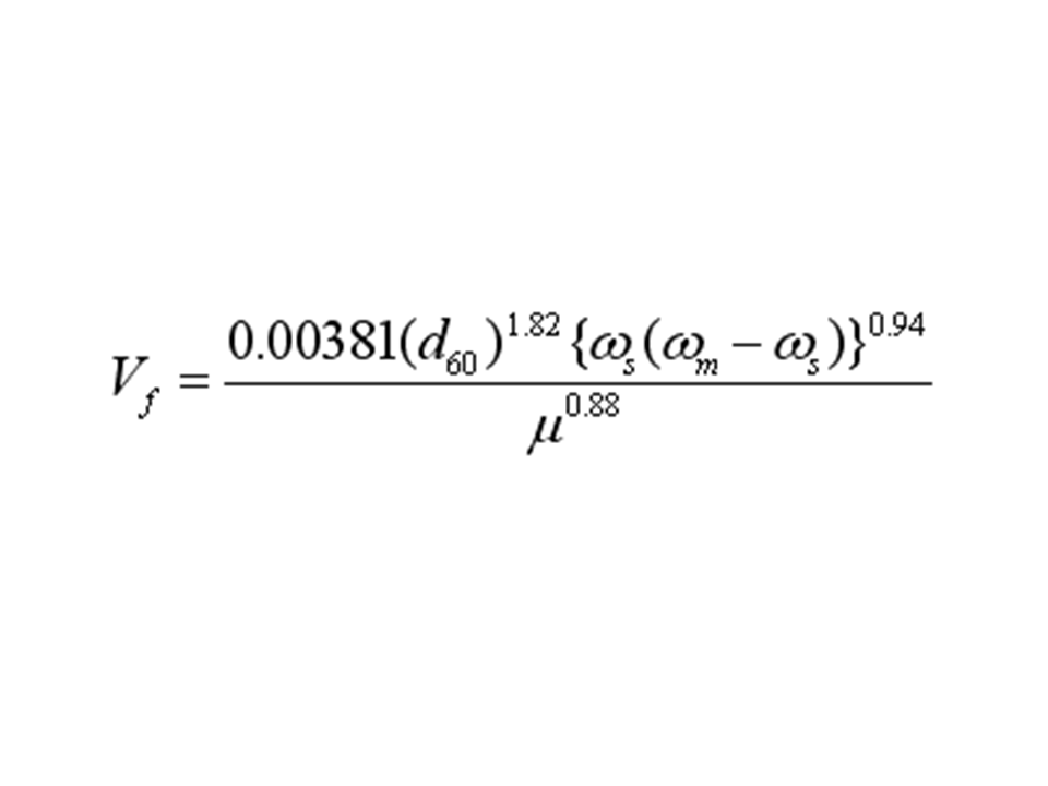
Then the velocity for backwash is based on the filtration velocity, the sand's porosity and the ratio of height of the expanded and unexpanded filter bed.
| Latex |
|---|
\large
$$
V = K_e (\overline \varepsilon  )^{n_e }
$$
|
| Latex |
|---|
\large
$$
\overline \varepsilon = 1 - {D \over {D_e }}(1 - \varepsilon )
$$
|
Once the back wash velocity is determined, solving the clear well and filter dimensions are the same process.
Design Output for Agalteca Plant, Q=6.3 L/s:
| Conservative | Empirical |
|---|---|---|
Filter Square Side | 1.5m | 1.5m |
Filter Height | 3.95m | 2.56m |
Clear Well Diameter | 6m | 6m |
Clear Well Height | 1.37m | 1.23m |
Mathcad Conclusions:
1) Our design based on simple hydraulics will work. However, it is a very large filter and will not be sustainable economically. The material cost for construction will be too high.
2) The design based on the empirical Weber equation (instead of the conservative approach) is much smaller and less expensive. We need to fine tune the material parameters we were using and make certain the equations were valid for our application. Also, the full validity of the empirical Weber equation is not certain.
3) If the empirical equations are valid, then we can change parts of the design, by changing the sand parameters. For example, lower BW velocity by lowering the d60 (diameter that 60% of the particles if less than or equal to) and specific weight of the media.
The basic concept of bench scale modeling is to test the effectiveness of an actual filtration design by shrinking the design parameters of the system (filter bed depth, filter bed surface area, and etc) to a smaller scale that is easier to test. For example, we would simulate a filter bed of 50 cm of sand with a 5 cm of sand with the porosity and specific gravity of the sand being constant. This would also enable us to test the validity of the empirical equations that are behind our design.
Our MATHCAD files are divided into three parts: input, calculation, and output. In the input section, the user is prompted to enter in the properties of the filter media, water, filter dimensions, and the degree of bed expansion targeted. The calculation section contains the empirical equations from Schulz, Okun, and Weber. The output section produces the fluidization velocity and the corresponding flow rate required for the targeted bed expansion.
Click here for the PDF version of our MATHCAD File.
Multiple Layer Media MATHCAD file is coming.