 Sign-up for free online course on ANSYS simulations!
| Include Page | ||||
|---|---|---|---|---|
|
| Include Page | ||||
|---|---|---|---|---|
|
Post Processing
Plot Velocity Vectors and Contours
| HTML |
|---|
<iframe width="560" height="315" src="https://www.youtube.com/embed/DCbh6z1v1wY" frameborder="0" allow="accelerometer; autoplay; encrypted-media; gyroscope; picture-in-picture" allowfullscreen></iframe> |
Note: In the below video (Plot Pressure Contours), please note that the cursor disappears accidentally at the 44 second mark and returns at the 3 minute mark. At 1 minute 17 seconds, "here" refers to the bottom-middle of the region near the plate. It is later drawn at the 1 minute 28 second mark. At 2 minute 40 seconds, "here" refers to the left most face, known as the inlet face, of the region.
Plot Pressure Contours
| HTML |
|---|
<iframe width="560" height="315" src="https://www.youtube.com/embed/KRQ0rtKCJ3w" frameborder="0" allow="accelerometer; autoplay; encrypted-media; gyroscope; picture-in-picture" allowfullscreen></iframe> |
Plot Velocity Profiles
| HTML |
|---|
<iframe width="560" height="315" src="https://www.youtube.com/embed/t3p52LPLw-A" frameborder="0" allow="accelerometer; autoplay; encrypted-media; gyroscope; picture-in-picture" allowfullscreen></iframe> |
Explanation for Velocity Profile Overshoot
| HTML |
|---|
<iframe width="560" height="315" src="https://www.youtube.com/embed/LnIsw07iuew?rel=0" frameborder="0" allowfullscreen></iframe> |
Check Similarity Principle
| HTML |
|---|
<iframe width="560" height="315" src="https://www.youtube.com/embed/Qde3pryaQ2A" frameborder="0" allow="accelerometer; autoplay; encrypted-media; gyroscope; picture-in-picture" allowfullscreen></iframe> |
Plot Velocity Derivatives
| HTML |
|---|
<iframe width="560" height="315" src="https://www.youtube.com/embed/kn6zk0AWsps" frameborder="0" allow="accelerometer; autoplay; encrypted-media; gyroscope; picture-in-picture" allowfullscreen></iframe> |
Calculate Drag Coefficient
| HTML |
|---|
<iframe width="560" height="315" src="https://www.youtube.com/embed/YrMyfB6n_W0" frameborder="0" allow="accelerometer; autoplay; encrypted-media; gyroscope; picture-in-picture" allowfullscreen></iframe> |
Go to Step 7: Verification & Validation
Go to all FLUENT Learning Modules
| Panel |
|---|
Author: John Singleton and Rajesh Bhaskaran, Cornell University Problem Specification |
| Note | ||
|---|---|---|
| ||
This page of this tutorial is currently under construction. Please check back soon. |
| Info | ||
|---|---|---|
| ||
Click here for the FLUENT 6.3 version. |
Step 6: Results
Velocity Vectors
...
https://confluence.cornell.edu/download/attachments/118771111/VectPlot_Full.png...
https://confluence.cornell.edu/download/attachments/118771111/VectPlot2_Full.pngOutlet Velocity Profile
...
https://confluence.cornell.edu/download/attachments/118771111/xyplotsetup_Full.png...
https://confluence.cornell.edu/download/attachments/118771111/SolXY1_Full.png...
https://confluence.cornell.edu/download/attachments/118771111/XVelPlot1_Full.png...
https://confluence.cornell.edu/download/attachments/118771111/AxesMen1_Full.png...
https://confluence.cornell.edu/download/attachments/118771111/Axes2_Full.png...
https://confluence.cornell.edu/download/attachments/118771111/Plot3_Full.png...
https://confluence.cornell.edu/download/attachments/118771111/Plot4_Full.pngPlot Pressure Coefficients
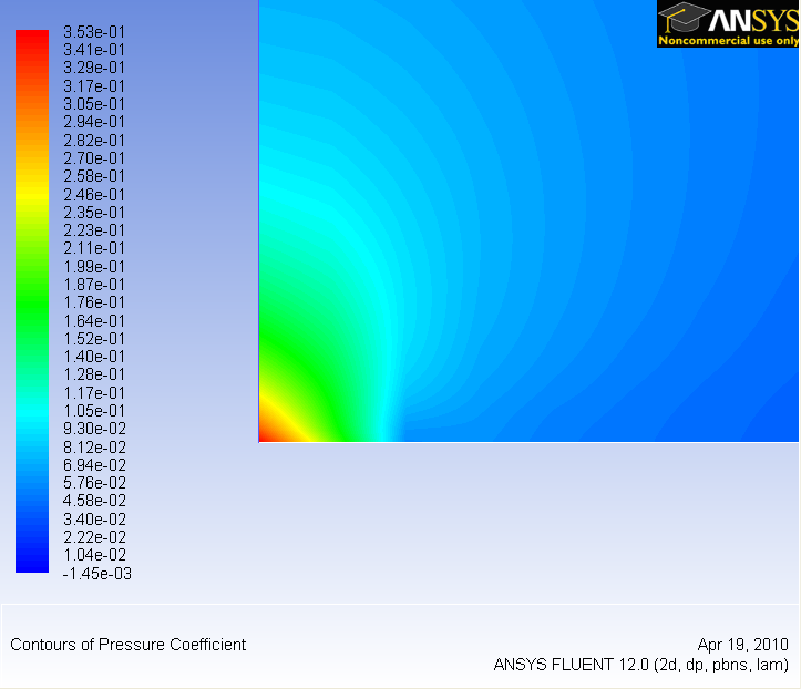
Now we will display the pressure coefficient contour but first we need to set the reference values for velocity. Go back to:
Problem Setup > Reference Values
And select inlet under Compute From. Then go back to:
Results > Graphics and Animations > Graphics > Contours
Select Pressure...under Contours Of. Then select Pressure Coefficient from the second drop-down menu. Also, check the Filled checkbox and set Levels to 90. Then click on Display to update the display window.
...
https://confluence.cornell.edu/download/attachments/118771111/step6_002.png?version=1Zoom in at the leading edge.
...
https://confluence.cornell.edu/download/attachments/118771111/step6_003.png?version=1Why is the pressure not constant at the leading edge of the plate?
Plot Skin Friction Coefficient
Now we will plot the skin friction coefficient along the flat plate.
Results > Plots > XY Plot
Change Pressure to Wall Fluxes. Then, change Wall Shear Stress to Skin Friction Coefficient. Under Surfaces, select plate.
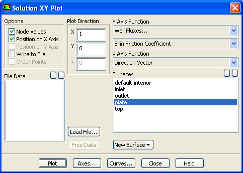
Click Plot.
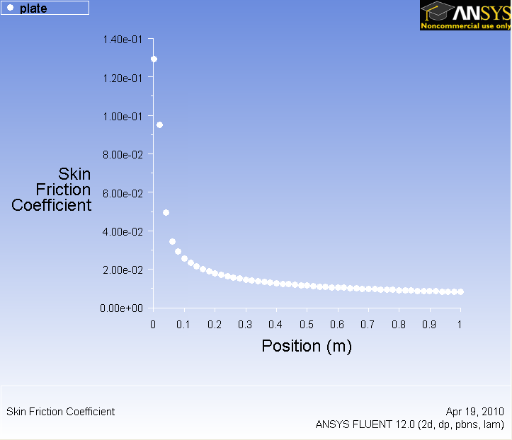
...
https://confluence.cornell.edu/download/attachments/118771111/step6_005.png?version=1Now, compare your solution to the with the Blasius solution's skin friction by loading the file and then plotting it with your solution. (Download file here)
...
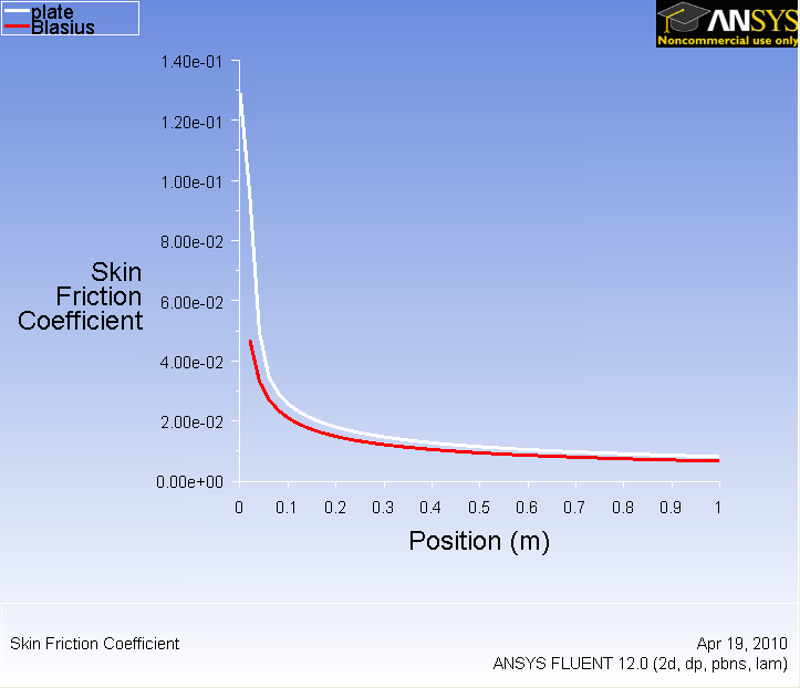
...
https://confluence.cornell.edu/download/attachments/118771111/step6_007.png?version=1Plot Velocity Profiles
Results > Plots > XY Plot
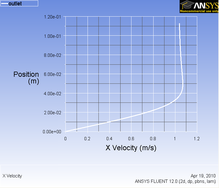
Uncheck Position on X Axis and check Position on Y Axis under Options. Under Plot Direction, set X to 0 and Y to 1. Under X Axis Function, select Velocity...Then, change Velocity Magnitude to X Velocity. Finally under surface, select outlet. Before we are ready to plot, click on the Axes... button and rescale the y-axis from 0 to 0.12. Also, check the Major Rules and Minor Rules for both axes. Remember that you must click the Apply button when performing changes in each axis.
Click Plot.
...
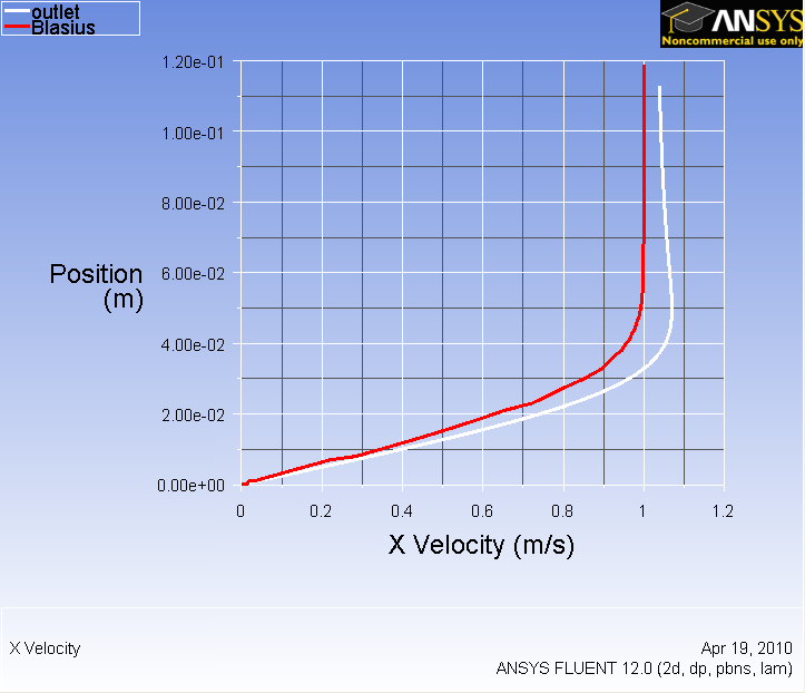
https://confluence.cornell.edu/download/attachments/118771111/step6_008.png?version=1To compare with the Blasius solution, download the solution here. Click Load File...and select the file you just downloaded. Then plot the solutions again to display both lines on the same graph.
...
https://confluence.cornell.edu/download/attachments/118771111/step6_009.png?version=1What is the noticeably different between two solutions? Why is the velocity overshoot 1 for FLUENT's solution?
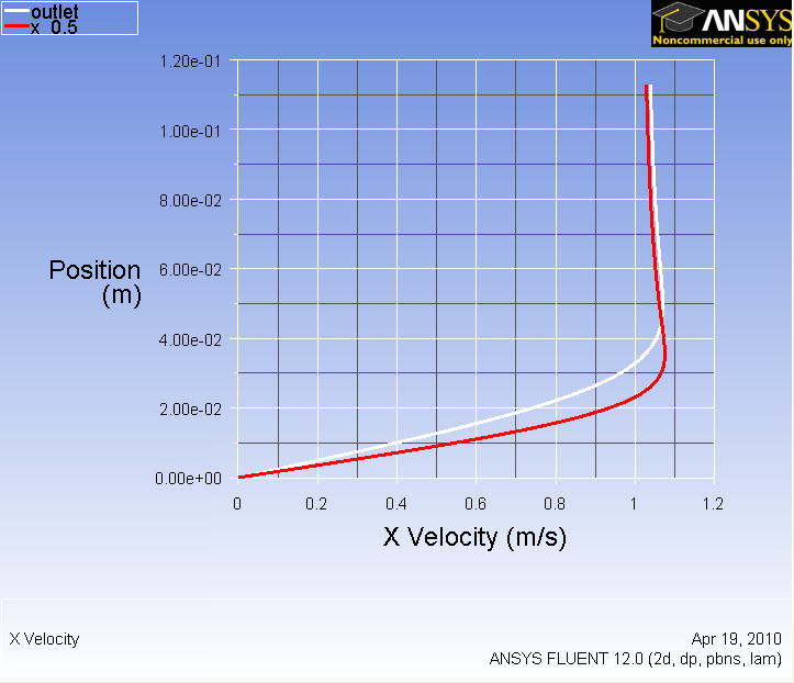
Now we will compare the velocity profile at two sections. Create another section in the middle of the plate.
Again, in the XY Plot window under New Surface > Line/Rake
Check the line tool checkbox under Options and set the initial coordinate to (0.5,0) and final coordinate to (0.5,0.5). Under the New Surface Name field, type in x_0.5 and then click the Create button to create the line.
We can now plot and compare the velocity profile at the mid point and the outlet of the flow.
Under Surfaces, select outlet and {}x_0.5 and Plot.
...
https://confluence.cornell.edu/download/attachments/118771111/step6_010.png?version=1Go to Step 7: Refine Mesh