 Sign-up for free online course on ANSYS simulations!
| HTML |
|---|
<div style="background-color: yellow; border: 2px solid red; margin: 4px; padding: 2px; font-weight: bold; text-align: center;">
This page has been moved to <a href="https://courses.ansys.com/index.php/courses/turbulent-pipe-flow-rans/">https://courses.ansys.com/index.php/courses/turbulent-pipe-flow-rans/</a>
<br>
Click in the link above if you are not automatically redirected in 10 seconds.
</div>
<meta http-equiv="refresh" content="10; URL='https://courses.ansys.com/index.php/courses/turbulent-pipe-flow-rans/'" />
|
| Include Page | ||||
|---|---|---|---|---|
|
| Include Page | ||||
|---|---|---|---|---|
|
Turbulent Pipe Flow
Created using ANSYS 13.0
| Note |
|---|
This tutorial has videos. If you are in a computer lab, make sure to have head phones. |
Problem
...
Specification
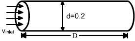
Let's revisit the pipe flow example considered in the previous exercise. As before, the inlet velocity is 1 m/s, the fluid exhausts into the ambient atmosphere and density is 1 kg/m3. For µ = 2 x 10^10 -5^ 5 kg/(ms), the Reynolds no. based on the pipe diameter and average velocity at the inlet is
| Latex |
|---|
\large
$$
{Re} = {\rho VD \over \mu} = 10,000
$$
|
This change of viscosity has taken us from a Reynolds number of 100 to 10,000. 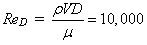
At this Reynolds number, the flow is usually completely turbulent. A turbulent flow exhibits small-scale fluctuations in time. It is usually not possible to resolve these fluctuations in a CFD calculation. So the flow variables such as velocity, pressure, etc. are time-averaged. Unfortunately, the time-averaged governing equations are not closed i.e. they contain fluctuating quantities which need to be modeled using a turbulence model. No turbulence model is currently available that is valid for all types of flows and so it is necessary to choose and fine-tune a model for particular classes of flows. In this exercise, you'll be turned loose on variants of the k-ε model. But in the real world, tread with great caution: you should evaluate the validity of your calculations using a turbulence model very carefully (which, ahem, means that there is no getting away from studying fluid dynamics concepts and numerical methods very carefully). FLUENT should not be used as a black box. The k-ε models consist of two differential equations: one each for the turbulent kinetic energy k and turbulent dissipation ε. These two equations have to be solved along with the time-averaged continuity, momentum and energy equations. So turbulent flow calculations are much more difficult and time-consuming than laminar flow calculations. This is an exercise to whet your appetite for turbulent flow calculations
We'll solve this problem numerically using ANSYS FLUENT. Among the results we'll look at are centerline velocity, skin friction coefficient and the axial velocity profile at the outlet.
Go to Step 1: Pre-Analysis & Start-Up
Go to all FLUENT Learning Modules Create Geometry in GAMBIT |