Page History

...

The real life flocculation tank designed by Aguaclara involved a 180 deg turn over few dozens baffles. For validating result and modeling purpose, a simple 180 deg turn over two baffles was modeled. The first step was to set up the geometry of the of the simple flocculator. For future comparison with the experimental data, the design parameters for the pilot plant test flocculator was modified and used. The modeling approach that was utilized was creating geometry, mesh geometry, setting boundary condition, and finally solving using FLUENT.

2.1 Creating Geometry 

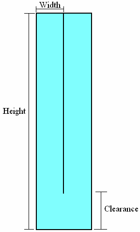
Figure 1: . Geometry of Flocculator

The design parameters used are:

...

With the geometry, the mesh for the model can then be set up.

2.2 Setting up Mesh 

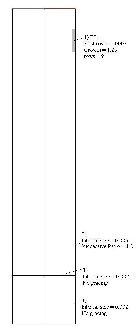
Figure 2: . Meshing Parameters (Click on the figure to see the original size)

 
Figure 2 shows the meshing parameters that were used. The boundary layers was first establish at all the wall surfaces. The boundary layer was set up such that the solution obtain in gambit would provide result of y+ of less than 5. After that, the mesh edges were set up such that they will provide higher mesh resolution near the turn and lower resolution far from the turn. With the initial meshing conditions set up, all the faces were then meshed.

 
   
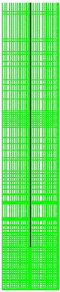
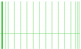
Figure 3: . Mesh of the Model (Click on figure for original size)

Figure 3 shows the overall mesh of the flocculator model. As can be seen, the mesh is fine near the turn and at the wall.  The final step at this point was to set up the boundary conditions of the system.

2.3 Setting up Boundary Conditions 

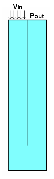
Figure 4: . Boundary Conditions

Figure 4 shows the boundary condition that was used for modeling. For a flocculator, there is an in flow and out flow of the fluids. Since inlet velocity inlet was known from the experimental data, the inlet was set to the Velocity Inlet type boundary condition. The outlet was set to Pressure Outlet boundary condition type, the atmospheric pressure.

...

The effect of number of mesh elements on the result was also carry out. Coarse mesh, medium mesh and fine mesh were created and the pressure drop across the turn from each mesh was compared. This analysis will provide confidence on the accuracy of certain mesh. If the changes in mesh elements does not result in a lot of change in pressure coefficient drop, it is concluded that the mesh elements is refine enough that the truncation error can be neglected. Following table Table 1 shows the summary of 3 meshes created for mesh sensitivity analysis. Please refer back to figure 2 for corresponding meshing parameters.

Table 1. Mesh Meshing Parameters for Coarse, Medium and Fine Mesh

...

At the later stage of project, after the good solution was obtained, the effect of geometry on results was analyzed. Different clearance height was used for analyzing new results as a result of this effect. It would be tedious to individually recreate each geometry and mesh for different clearance height from scratch. For this reason, parameterization technique was used. The original Gambit journal file was modified to include the variable clearance height. Using this method, changes in corresponding clearance height was plug into the journal file and run using Gambit to obtain desired mesh and geometry. The journal files used for such parameterization is included in the Appendix.

2.6 Comparing Turbulence Model

Different turbulence model were also used

...

Some of the important results are the velocity vectors, contour of pressure coefficient, contours of pressure coefficient, contours of strain rate and contours of turbulence dissipation rate.

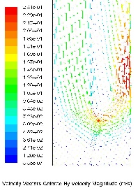
Figure 5: . Velocity Vectors (Click on figure for original size)
 
Velocity vector plot shows the velocity of the fluids throughout the flocculator.  As can be seen, there is a region of high velocity at the outer turn and recirculation at the inner turn. At the bottom of the flocculator, there is region of stagnant fluid.
 

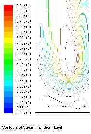
Figure 6: . Contours of Stream Function (Click on figure for original size)
 
Contours of stream function tell us how the fluid travel in the flocculator. As can be seen from figure 6, there is enclosed streamline at the inner turn. The enclosed streamlines means there are recirculating fluid which are trapped in the region.

 
 

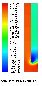
Figure 7: . Contours of Pressure Coefficient

Figure 7 shows most of the pressure coefficient drop occurs around the bend. There is a pressure coefficient drop of about 3.7 across the bend. (Talk about the experimental result. Literature review data)

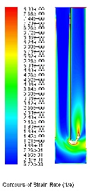
Figure 8: . Contours of Strain Rate

Contours of strain rate shows high strain rate right before and after the turn. There are also high strain rate near the wall. The region with high strain rate is the region where the flocculation occurs.

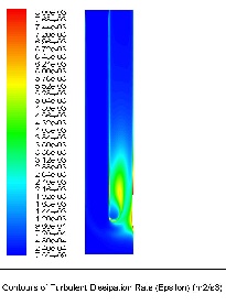
Figure 9: . Contours of Turbulent Disssipation Rate

Contours of turbulent dissipation rate shows about the same trend as the contours the strain rate right after the turning. The region of high turbulence dissipation after the turn is about twice the length of baffle spacing (research literature). The high dissipation rate after the turn is because of the expansion of the fluid.

...