 Sign-up for free online course on ANSYS simulations!
| Wiki Markup |
|---|
{alias:pipe2}
{panel}
|
| Panel |
Author: Rajesh Bhaskaran, CornellUniversity Problem Specification |
Problem Specification
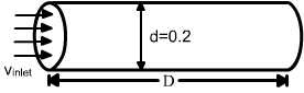
Let's revisit the pipe flow example considered in the previous exercise. As before, the inlet velocity is 1 m/s, the fluid exhausts into the ambient atmosphere and density is 1 kg/m3. For µ = 2 x 10^-5^ kg/(ms), the Reynolds no. based on the pipe diameter and average velocity at the inlet is
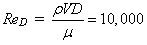
At this Reynolds number, the flow is usually completely turbulent.
A turbulent flow exhibits small-scale fluctuations in time. It is usually not possible to resolve these fluctuations in a CFD calculation. So the flow variables such as velocity, pressure, etc. are time-averaged. Unfortunately, the time-averaged governing equations are not closed i.e. they contain fluctuating quantities which need to be modeled using a turbulence model. No turbulence model is currently available that is valid for all types of flows and so it is necessary to choose and fine-tune a model for particular classes of flows. In this exercise, you'll be turned loose on variants of the k-ε model. But in the real world, tread with great caution: you should evaluate the validity of your calculations using a turbulence model very carefully (which, ahem, means that there is no getting away from studying fluid dynamics concepts and numerical methods very carefully). FLUENT should not be used as a black box. The k-ε models consist of two differential equations: one each for the turbulent kinetic energy k and turbulent dissipation ε. These two equations have to be solved along with the time-averaged continuity, momentum and energy equations. So turbulent flow calculations are much more difficult and time-consuming than laminar flow calculations. This is an exercise to whet your appetite for turbulent flow calculations.
Go to Step 1: Create Geometry in GAMBIT
See and rate the complete Learning Module
...
 University

{color:#ff0000}{*}Problem Specification{*}{color}
[1. Create Geometry in GAMBIT|FLUENT - Turbulent Pipe Flow - Step 1]
[2. Mesh Geometry in GAMBIT|FLUENT - Turbulent Pipe Flow - Step 2]
[3. Specify Boundary Types in GAMBIT|FLUENT - Turbulent Pipe Flow - Step 3]
[4. Set Up Problem in FLUENT|FLUENT - Turbulent Pipe Flow - Step 4]
[5. Solve!|FLUENT - Turbulent Pipe Flow - Step 5]
[6. Analyze Results|FLUENT - Turbulent Pipe Flow - Step 6]
[7. Refine Mesh|FLUENT - Turbulent Pipe Flow - Step 7]
[Problem 1|FLUENT - Turbulent Pipe Flow - Problem 1]
{panel}

h2. Problem Specification

!Fluent_pipeflow.jpg!

Let's revisit the pipe flow example considered in the previous exercise.          As before, the inlet velocity is 1 m/s, the fluid exhausts into the ambient          atmosphere and density is 1 _kg/m{_}{_}{^}3{^}_. For µ = 2          x 10^-5\^ _kg/(ms_), the Reynolds no. based on the pipe diameter          and average velocity at the inlet is

 !Fluent_Eq2.jpg!

At this Reynolds number, the flow is usually completely turbulent.

A turbulent flow exhibits small-scale fluctuations in time. It is usually          not possible to resolve these fluctuations in a CFD calculation. So the          flow variables such as velocity, pressure, etc. are time-averaged. Unfortunately,          the time-averaged governing equations are not closed i.e. they contain          fluctuating quantities which need to be modeled using a turbulence model.          No turbulence model is currently available that is valid for all types          of flows and so it is necessary to choose and fine-tune a model for particular          classes of flows. In this exercise, you'll be turned loose on variants          of the _k-ε_ model. But in the real world, tread with great _caution_: you should evaluate the validity of your calculations          using a turbulence model very carefully (which, ahem, means that there          is no getting away from studying fluid dynamics concepts and numerical          methods very carefully). FLUENT should _not_ be used as a black          box. The _k-ε_ models consist of two differential equations:          one each for the turbulent kinetic energy _k_ and turbulent dissipation ε.          These two equations have to be solved along with the time-averaged continuity,          momentum and energy equations. So turbulent flow calculations are much          more difficult and time-consuming than laminar flow calculations. This          is an exercise to whet your appetite for turbulent flow calculations.

Go to [Step 1: Create Geometry in GAMBIT|FLUENT - Turbulent Pipe Flow - Step 1]

[See and rate the complete Learning Module|FLUENT - Turbulent Pipe Flow]

Go to [all FLUENT Learning Modules|FLUENT Learning Modules] |